Chaire d'Analyse Appliquée                    The DNA modelling COURSE

Session 4

Introduction

We have introduced the kinematics, balance laws, and simple linear constitutive relations for a special Cosserat rod deforming in three dimensions, for both shearable, extensible rods, and for inextensible, unshearable rods.

In the exercises, you have considered some simple equilibria when the rod is uniform (i.e. the constitutive relations have no explicit dependence on the parameter $s$ ) that can be calculated analytically in closed form. However for non-uniform rods, and for many two-point boundary value problems for rods it is necessary to use numerics to determine the equilibria.

We now turn to start a description of the combination of analysis and numerical methods that we will use to compute equilibria that model DNA.

For various reasons, for example handling boundary conditions efficiently, constructing explicit variational principles, it can sometimes be convenient to explicitly parametrize the directors $\{\d_i(s)\}$, which, as previously remarked, is equivalent to parametrizing the group of proper rotation matrices or $SO(3)$. The classic choice (as described in nauseating detail in infinitely many mechanics texts) for such a parametrization is some set of Euler angles. We will later describe a parametrization in terms of Euler parameters (or, more or less equivalently, quaternions or Cayley-Klein parameters). However the kinematics of $SO(3)$ is unavoidably complicated in some ways.

Consequently, so as to focus first on the mathematical and computational techniques that are pertinent to our study of rods we will start with a study of the much simpler case involving planar (untwisted) deformations of rods. We will seek solutions of the full three dimensional equilibrium equations, which happen to be untwisted and to lie in a plane.

The planar rod example

That is (for example with deformations chosen to lie in the $(\i_1,\i_3)$ plane) $${\bf r}'\cdot\i_2 = 0 \quad \d_2(s)\equiv\i_2$$ or equivalently $$v_2(s)\equiv 0$$ and the Darboux vector has the simple form $$\u= u_2\d_2 = u_2\i_2$$ For such directors we can parametrize with a single angle $\phi(s)$ $$\d_1 = \cos\phi\,\i_1 - \sin\phi\,\i_3,\quad\d_3 = \sin\phi\,\i_1 +\cos\phi\,\i_3\,.$$ With this sign convention we find $\d_1=\i_1$ and $\d_3=\i_3$ when $\phi=0$ and moreover $$u_2\equiv +\phi'$$ (In the $(\i_1,\i_3)$-plane positive $\phi$ then corresponds to a clockwise rotation of the $\d_i$, see figure.) It is then easy to verify that provided $$\hat v_2\equiv 0\qquad\hat u_1\equiv \hat u_3\equiv 0,$$ with the diagonal constitutive relation introduced earlier, such planar kinematics generates forces and moments of the special form $${\bf n}\cdot \i_2\equiv 0 \qquad {\bf m}(s)\equiv m_2(s)\i_2$$ That is, the out of plane component of the force ${\bf n}$ vanishes, while the two in-plane components of the moment ${\bf m}$ vanish.

Notice that in general $m_2(s)$ denotes the component of ${\bf m}$ with respect to the director frame, but with the special kinematics introduced here $\d_2(s)\equiv\i_2$, so that $m_2(s)$ is also the component of ${\bf m}$ with respect to the fixed vector $\i_2$. Are there equilibria of this special form? To investigate this question we merely substitute our ansatz into the balance laws.

We find that the $2$-component of the force balance law is automatically satisfied, while both the $\d_1$ and $\d_3$ components (or equivalently here, both of the in-plane components $\i_1$ and $\i_3$) of the moment balance law are automatically satisfied.

The remaining system involves two scalar equations for the in-plane components $(n_1,n_3)$ of the force ${\bf n}$ and a third scalar equation for the out-of-plane component $m_2$ of the moment ${\bf m}$, Using the parametrization $\phi(s)$ of the directors, these equations can be written in the form

$$n_1'= -n_3\phi'\qquad n_3'=\phi'n_1,$$
$$m_2'= n_3v_1 - n_1v_3.$$

As we shall see in a moment, it can be convenient for the treatment of boundary conditions to retain the angle $\phi(s)$ as one of our basic unknowns. Thus we shall eliminate $m_2$ through the constitutive relation for bending which takes the form

$$m_2 = K_2(s)(\phi'-\hat u_2(s))$$ where as before $K_2(s)\gt$ and $\hat u_2(s)$ are given functions. The above equations form a closed system when two of the four unknowns $n_1$,$n_3$, $v_1$, and $v_3$ are eliminated through the use of the shear and extension constitutive relations (or, equivalently, the shear and extension constitutive relations are appended as additional equations)

We shall be primarily concerned with the inextensible, unshearable case in which the basic unknowns are $\phi$, $n_1$ and $n_3$ and

$$v_1\equiv\hat v_1\equiv 0,\qquad v_3\equiv\hat v_3\equiv 1.$$ and the governing equations reduce to $$n_1'= -n_3\phi'\qquad n_3'=\phi'n_1,$$
$$[K_2(s)(\phi'-\hat u_2(s))]'= -n_1.$$
$${\bf r}'=\d_3 = \sin\phi\,\i_1 +\cos\phi\,\i_3\,.$$ For this system it is actually more traditional to introduce the components $N_1$ and $N_3$ of the force ${\bf n}$ with respect to the fixed basis vectors $\i_1$ and $\i_3$. Because the angle $\phi$parametrizing the directors is one of our basic unknowns it is easy to achieve this explicitly through the invertible relationships (just familiar formulas from rotations in two-dimensions) $$n_1 = N_1\,\cos \phi - N_3\,\sin \phi \,,$$
$$n_3= N_1\,\sin \phi + N_3\,\cos \phi.$$ Then (verify this!) the governing equations reduce to $$N_1'= 0\, ,\qquad N_3'= 0,$$
$$[K_2(s)(\phi'-\hat u_2(s))]'= N_3\,\sin \phi - N_1\,\cos \phi$$
$${\bf r}'=\d_3 = \sin\phi\,\i_1 +\cos\phi\,\i_3\,.$$ which can be viewed as a single second-order ODE for the angle $\phi$,containing two unknown constants $N_1$ and $N_2$ (but not the centerline ${\bf r}$), along with a quadrature to determine ${\bf r}$ once $\phi$ is known.

This decoupling into an equation for $\phi$ plus unknown constants, and a quadrature for ${\bf r}$ can be rather convenient, and is one of the reasons that we introduce a parametrization of the director frame $\{\d_i\}$.However it turns out that the decoupling only truly works for certain sets of boundary conditions. We will first consider a set of boundary conditions for which there is a genuine decoupling.

The strut boundary conditions for an inextensible, unshearable rod of arc-length $1$ are

$$\phi(0)=0,\quad m_2(1)\equiv K_2(\phi'-\hat u_2)\vert _{s=1}=0,$$
$$N_3(1) = -\lambda,\quad N_1(1)=0$$
$${\bf r}(0)=0$$ Here $\lambda$ is a parameter (either positive or negative) which is specified. It represents the end-loading. The introduction of the minus sign is a convention meaning that the end-load is positive if the load is down the $\i_3$ axis.

More generally all the boundary conditions could have parameters on the right hand side instead of zero, although there is no interest in introducing additional parameters that merely generate planar rigid body motions of other solutions (e.g. parameters in the initial values for ${\bf r}(0)$ and $\phi(0)$, in addition to parameters for both $N_3(1)$ and $N_1(1)$).

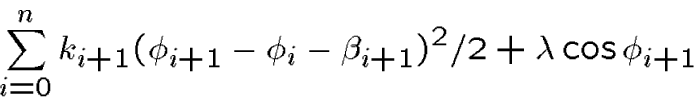
We will shortly introduce a discretization of the above two-point boundary value problem, which will lead to a discrete nonlinear system to be solved numerically. Actually we will introduce two different discretizations-a numerically naive one (a very rudimentary finite difference scheme) which we will use to explain the numerical solution procedures, and a numerically robust one (collocation) which we will compute with.

The computations will be carried out with a software package called VBM for solving the system obtained after discretization via collocation. VBM is a nice GUI and visualization package that in turn implements a continuation and bifurcation package called AUTO to generate numerical approximations to the solutions of the equilibrium boundary value problem.

We will use VBM as a black box (or at least a very dark grey box) code, first for the simple planar problem being considered now, and later for rod models more closely related to DNA. There will be no need for previous experience in programming (although if you have experience you will be able to do lots of extra nice things with VBM).

The first step is to discuss what bifurcation and continuation algorithms are, in order to have some idea about the output of the code.

We start with continuation algorithms for solving parameter dependent problems. And the first step in any continuation algorithm, is an explicitly known solution at some simple set of parameter values.

In what circumstances does the planar rod problem above have a simple explicit solution?

Recall that the balance laws are

$$N_1'= 0\, ,\qquad N_3'= 0,$$
$$[K_2(s)(\phi'-\hat u_2(s))]'= N_3\,\sin \phi - N_1\,\cos \phi$$
$${\bf r}'=\d_3 = \sin\phi\,\i_1 +\cos\phi\,\i_3\,.$$
 

One case in which there is a simple solution is when $\lambda=0$. Then

$$N_1(s) \equiv N_3(s)\equiv 0,$$
$$\phi(s)\equiv \int_0^s\hat u_2(\sigma)\,d\sigma\quad{\bf r}(s)\equiv\int_0^s\cos\phi(\sigma)\,d\sigma.$$

Recall that the strut boundary value problem had the boundary conditions

$$\phi(0)=0,\quad {\bf r}(0)=0$$ and $$N_3(1) = -\lambda,\quad N_1(1)=0\,,$$
$$\quad m_2(1)\equiv [K_2(\phi'-\hat u_2)]\vert _{s=1}=0,$$ where we have re-grouped the boundary conditions firstly into kinematic conditions, and secondly into external loading conditions.

Notice that we have used all of the boundary conditions in deriving the explicit representation of the solution to the boundary value problem.

Such a representation is called a solution by quadrature--all the variables are given in terms of indefinite integrals of known functions with explicit limits. In some sense the solution is not truly explicit unless the function $\hat u_2(s)$ is simple enough that the quadratures can be carried out in closed form (e.g. $\hat u_2$ a constant) but that is rarely important. For example continuation codes could easily use such a quadrature representation to generate a discretized solution of any required accuracy to use as a starting point.

The quadrature representation also contains interesting physical information. When all external loading vanishes, i.e. $\lambda=0$ in the above, then the rigid body transformation of the unstressed, minimum-energy shape that is uniquely defined by the kinematic boundary conditions is a solution of the equilibrium conditions.

Less obviously the constructive nature of the quadrature solution demonstrates that it represents the unique solution of the boundary value problem. Whenever $\lambda$ is non-zero it is much harder to obtain such a uniqueness result. Indeed unless $\vert\lambda\vert$ is sufficiently small, the boundary value problem has multiple solutions, and there is no uniqueness.

Exercise: What can be said about existence and uniqueness of solutions when the external loading conditions are assumed to be of the form

$$N_3(1) = 0,\quad N_1(1)=0\,,$$
$$\quad m_2(1)\equiv [K_2(\phi'-\hat u_2)]\vert _{s=1}=\tau,$$ i.e. no external force loading at the end, but instead an external torque loading $\tau\d_2$?

We will re-visit uniqueness (and non-uniqueness) results later after a variational formulation of the problem has been introduced and convexity arguments can be brought to bear.

We will also have need of another special case, namely when $\hatu_2(s)\equiv 0$. Then the equilibrium equations reduce to

$$N_1'= 0\, ,\qquad N_3'= 0,$$
$$[K_2(s)\phi'\,]'= N_3\,\sin \phi - N_1\,\cos \phi$$
$${\bf r}'=\d_3 = \sin\phi\,\i_1 +\cos\phi\,\i_3\,.$$

and we see that there is a whole family of solutions satisfying the strut boundary conditions, namely

$$\phi(s)\equiv 0, \quad N_1=0,\quad N_3=-\lambda$$
$${\bf r}(s)= s\,\i_3$$ which is a solution for all values of the parameter $\lambda$.

 Physically this means that when you lean straight down on a perfectly straight, inextensible (or in this case incompressible), upright rod, then the undeformed configuration is an equilibrium for any load. What does your intuition tell you will happen for sufficiently large loads? Well the strut will start bending (or in another description will buckle). Or perhaps compression effects will become non-negligible (depending on the material or constitutive relation). Thus we see that in a parameter dependent problem we always have to be aware of limitations of the range and idealizations of the model. In point of fact the inextensible model captures the phenomenon of buckling rather well through the phenomena of bifurcation and an associated loss of stability, and also through the inclusion of imperfections (for example the presence of a rather small $\hat u_2(s)$ representing a nearly straight unstressed shape). Both buckling and imperfections will be crucial in the DNA minicircle example.

To understand buckling and imperfections we will retreat to an even simpler finite dimensional model, which can be regarded as a finite difference approximation to the planar rod problem. Consider the energy

$$\sum_{i=0}^n k_{i+1} (\phi_{i+1} - \phi_i -\beta_{i+1})^2/2 + \lambda \cos\phi_{i+1}$$

 Back to the Table of Contents